graph-sto-iht

Stochastic IHT for Graph-structured Sparsity Optimization

Overview

Welcome to the repository of GraphStoIHT! This repository is only for reproducing all experimental results shown in our paper. To install it via pip, please try sparse-learn. Our work is due to several seminal works including StoIHT, AS-IHT, and GraphCoSaMP. More details of GraphStoIHT can be found in: “Baojian Zhou, Feng Chen, and Yiming Ying, Stochastic Iterative Hard Thresholding for Graph-structured Sparsity Optimization, ICML, 2019”.

Our code is written in Python and C11. The implementation of head and tail projection are almost directly from Dr. Ludwig’s excellent code cluster_approx, graph_sparsity and pcst_fast. I used C to reimplement these two projections is to get a little bit faster speed by using continuous memory (but the improvement is not significant at all!). As we pointed in sparse-learn, you can install GraphStoIHT via the following command:

$ pip install sparse-learn

After install it, you can use it via the following python interface

import splearn as spl

Instructions

The code has been tested on a GNU/Linux system. The dependencies of our programs are Python2.7(with numpy) and GCC. This section is to tell you how to prepare the environment. It has four steps:

0.  clone our code website: git clone https://github.com/baojianzhou/graph-sto-iht.git

1.  install Python-2.7 and GCC (Linux/MacOS/MacBook users skip this!)

2.  install numpy, matplotlib (optional), and networkx (optional).

3.  after the above three steps, run: python setup.py build_ext --inplace.

After step 3, it will generate a sparse_module.so file. We are ready to show/replicate the results reported in our paper.

1. Figure 1

Figure 1 shows the subgraphs used in graph sparse linear regression. To generate Figure-1, run:

$ python exp_sr_test01.py gen_figures

Four figures will be generated in results folder. We show the four generated figures in the following.

Graph with sparsity 8	Graph with sparsity 20	Graph with sparsity 28	Graph with sparsity 36

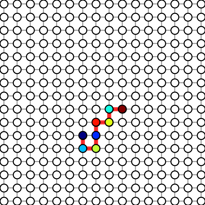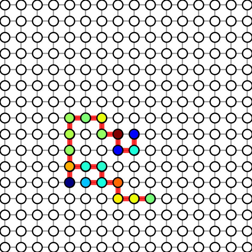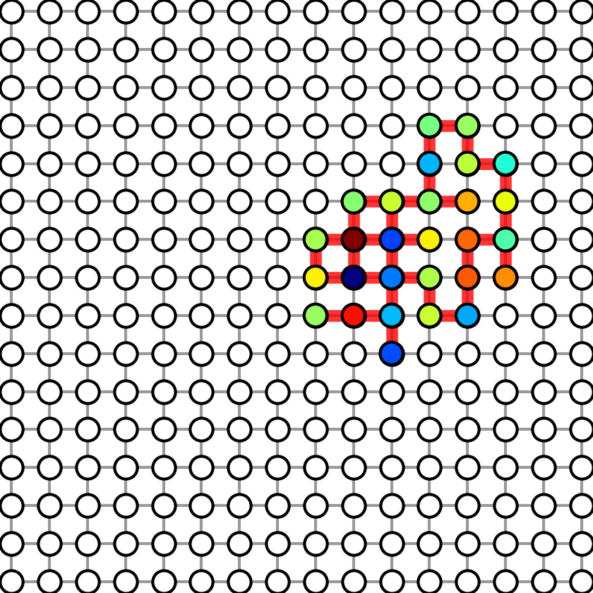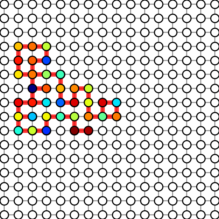2. Figure 2

To show Figure-2, run:

$ python exp_sr_test02.py show_test

To reproduce Figure-2, run:

$ python exp_sr_test02.py run_test 4

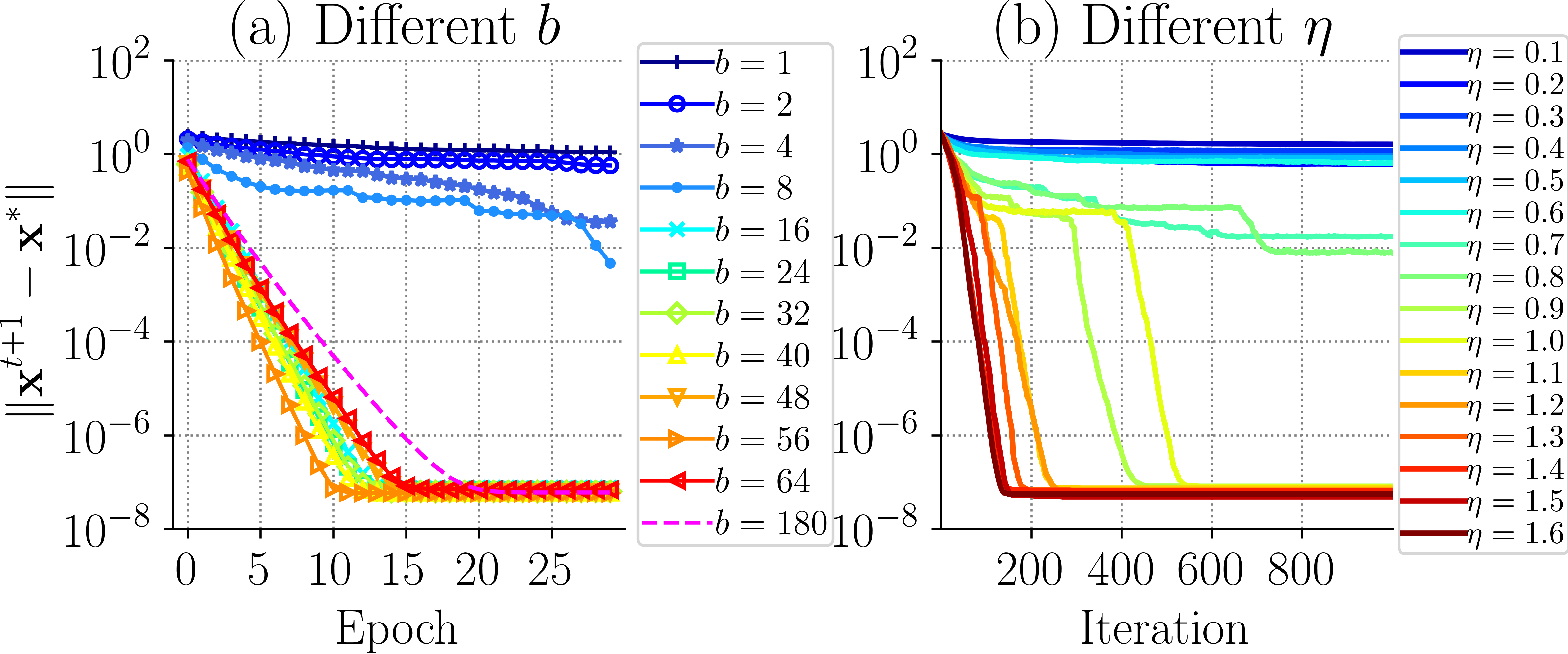
Here, the parameter 4 is the number of CPU will be used. The left illustrates the estimation error as a function of epochs for different choices of b. When b= 180, it degenerates to GraphIHT (the dashed line). The right part shows the estimation error as a function of iterations for different choices of η. It shows that when the sample size is suitable, the algorithm converges faster than batch method.

3. Figure 3

To show Figure-3, run:

$ python exp_sr_test03.py show_test

To reproduce Figure-3, run:

$ python exp_sr_test03.py run_test 4 0 50

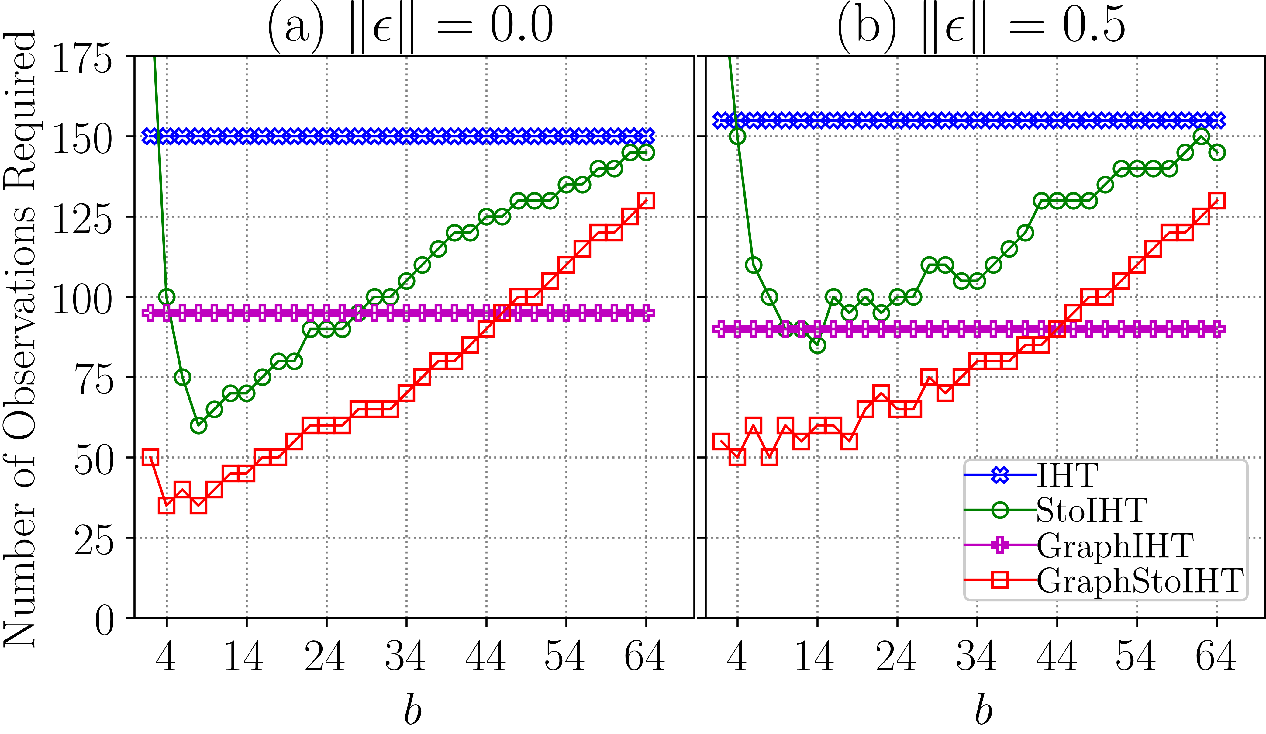
Here, 4 is the number of CPUs used for each program. 0 is the start of the trial id. 50 is the end of the trial id. It means we try to run 50 trials and then take the average. The figure shows the robustness to noise. The number of observations required is a function of different block sizes.

4. Figure 4

To show Figure-4, run:

$ python exp_sr_test01.py show_test

To reproduce Figure-4, run:

$ python exp_sr_test01.py run_test 4 0 50

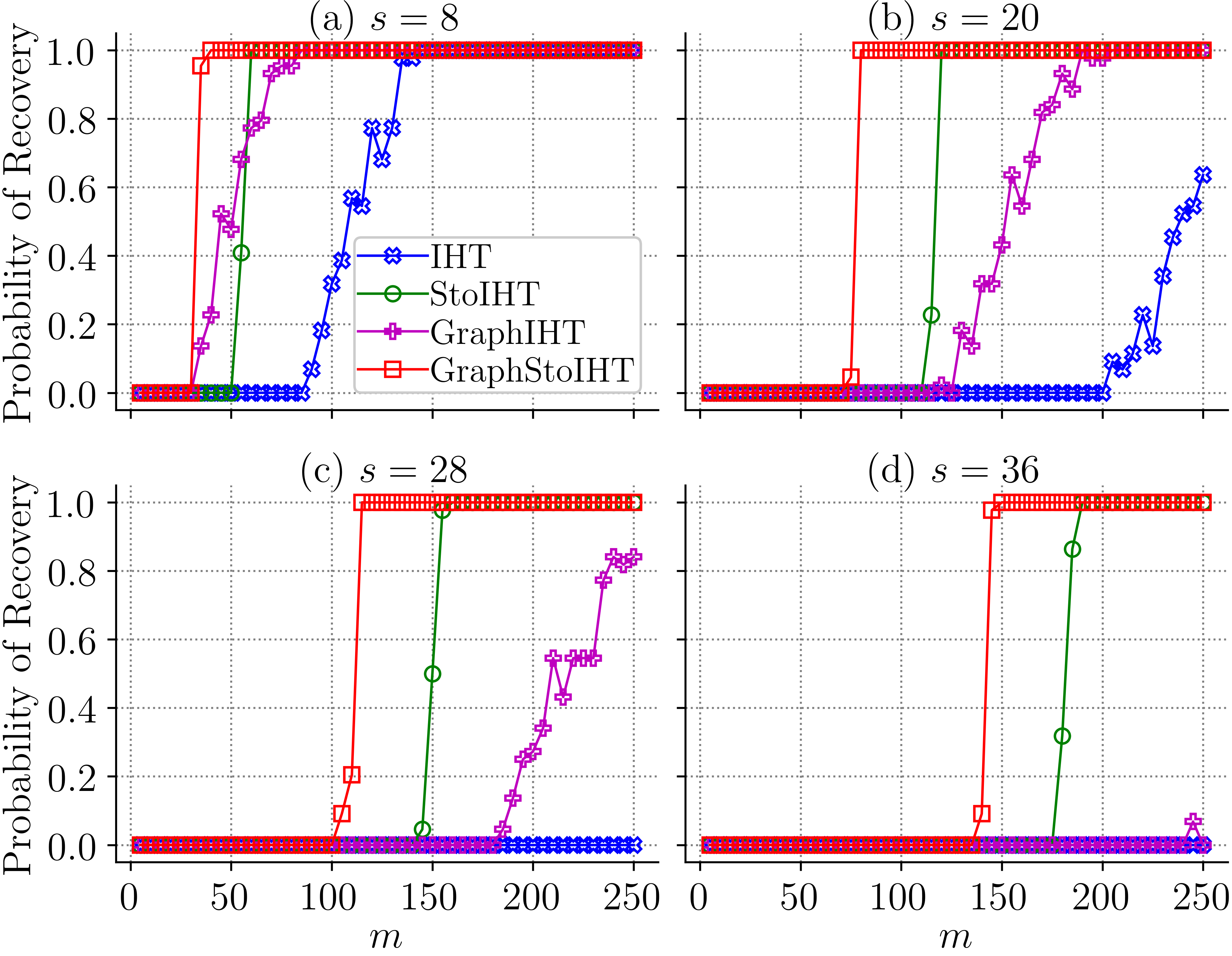
Here, 4 is the number of CPUs used for each program. 0 is the start of the trial id. 50 is the end of the trial id. It means we try to run 50 trials and then take the average. The figure shows the probability of recovery on synthetic dataset. The probability of recovery is a function of the number of observations m.

5. Figure 5

To show Figure-5, run:

$ python exp_sr_test06.py show_test

To reproduce Figure-5, run:

$ python exp_sr_test06.py run_test 4 0 50

Here, 4 is the number of CPUs used for each program. 0 is the start of the trial id. 50 is the end of the trial id. These three images are from graph-sparsity. We resize them to 50x50.

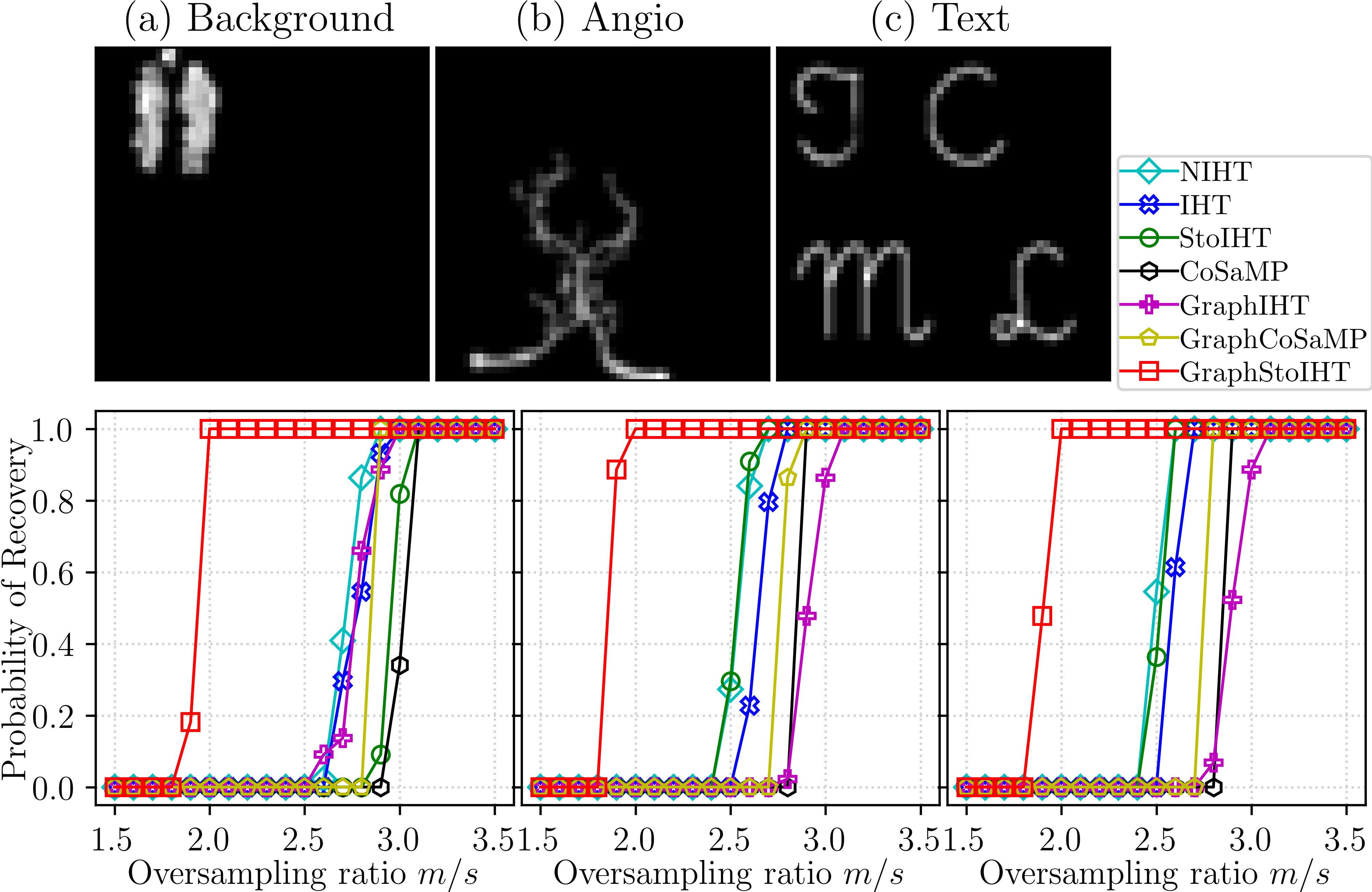
Probability of recovery on three 50×50 resized real im-ages.

6. Figure 6

To show Figure-6, run:

$ python exp_sr_test04.py show_test

To generate results of Figure-6, run:

$ python exp_sr_test04.py run_test 4 0 50

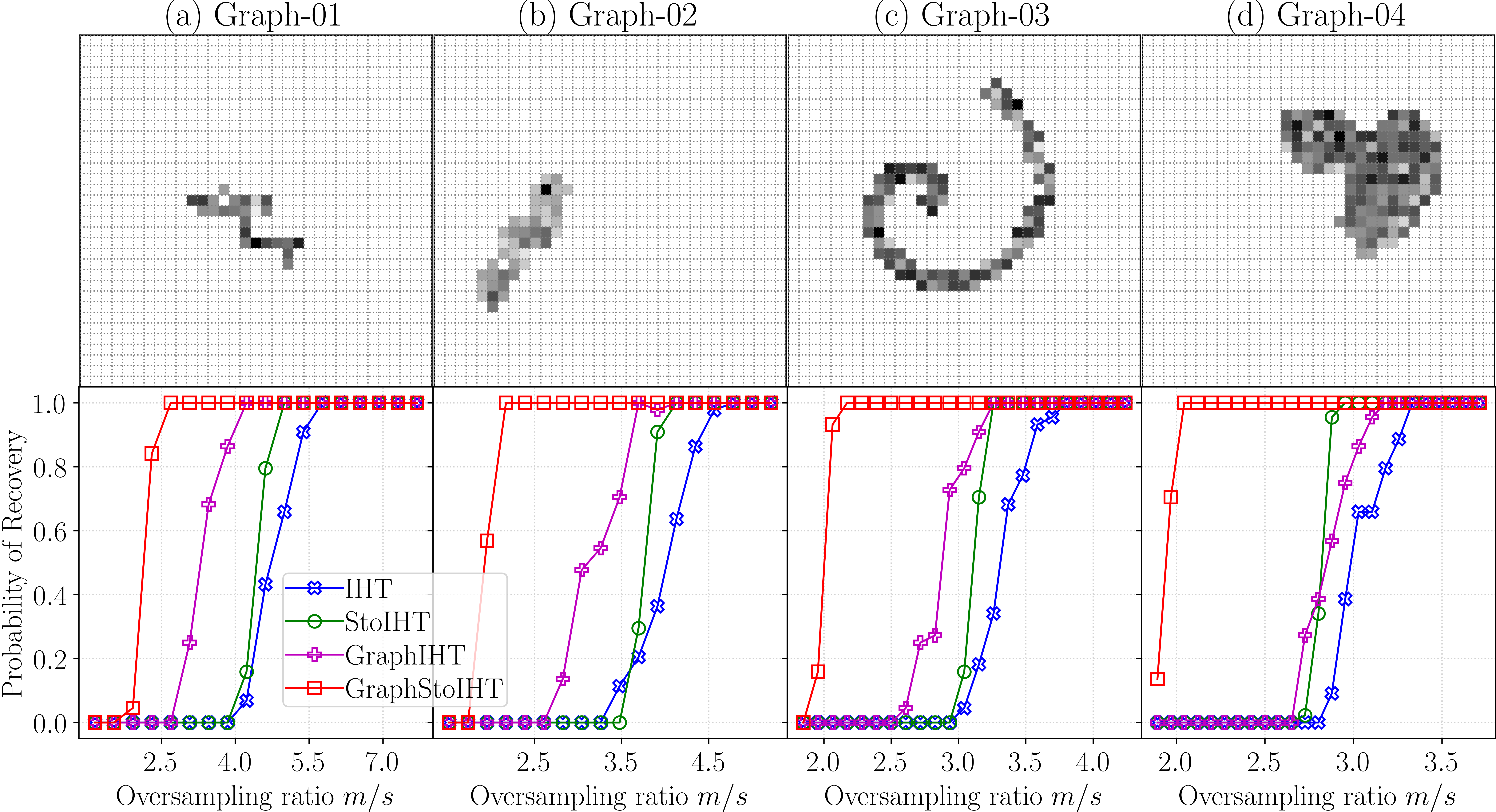
The probability of recovery as a function of oversampling ratio. The oversampling ratio is defined as the number of observations m divided by sparsity s, i.e.,m/s. These four public benchmark graphs (a), (b), (c), and (d) in the upper row are from Arias-Castro et al.(2011).

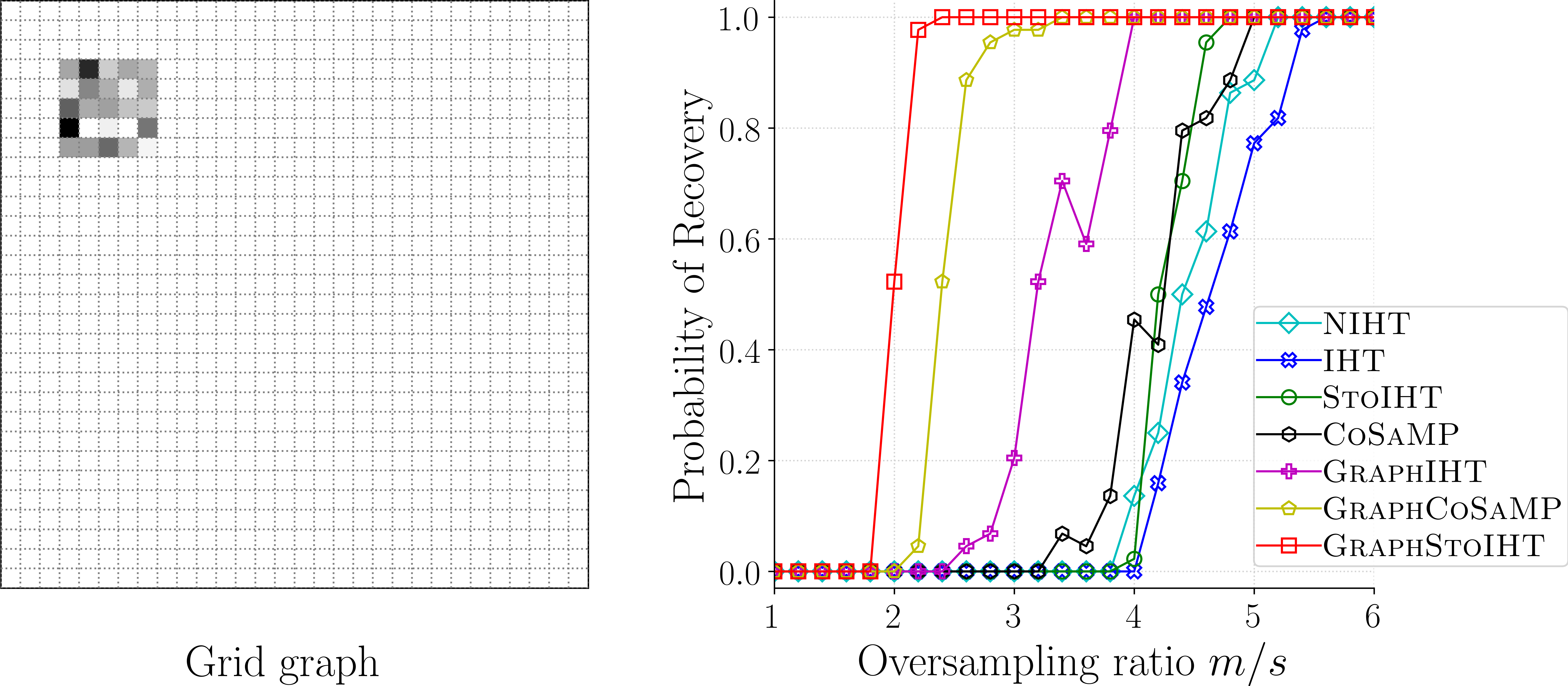
7. Figure 7

To show Figure-7, run:

python exp_sr_test05.py show_test

To generate results of Figure-7, run:

python exp_sr_test05.py run_test 4 0 50

8. Figure 8

To generate Table 2, 3, 4, 5, run: python exp_bc_run.py show_test

This section describes how to reproduce the results. In the following commands, –4 means the number of cpus used for each program. –0 means the start of the trial id. –50 means the end of the trial id.

To generate results of Table 2, 3, 4, 5, run: python exp_bc_run.py run_test 0 20

L1/L2-based methods

How to run l1/l2-mixed norm methods? You can first download Overlasso. We downloaded it in overlasso-package. Run those l1/l2-mixed norm methods 20 times and then generate the data and results in results folder.

Concerns and Issues

This section describes how to run GraphStoIHT and all baselines. The $\ell_1$ norm-based method is downloaded from OverLasso. It contains all l1/l2 mixed-norm methods. Since we reported results based 50 trials, some programs above are time-cost if you only use 4 CPUs. A better way is to test them on 5/10 trials by replacing 50 with 5/10. You should be approximately able to reproduce our results. If you cannot reproduce the results pleased email: bzhou6@albany.edu. We can discuss any concerns and potential issues could occur. Thank you in advance!

This section describes